North Reading Engineering

INTRODUCTION
When confronted with projects that require impedance analysis, the engineer has no better friend than Microsoft Excel. Here, I'll show how to make sense of impedance magnitude and phase angle measurements and how Excel can be used to generate a Nyquist plot like the one shown above. Note that measuring the complex impedance of a loudspeaker system, across a range of frequencies, requires dedicated measurement hardware. This brief doesn't consider how to measure the impedance but assumes that frequency dependent impedance magnitude and phase angle data is available for analysis.

Where impedance analysis has value is in modeling loudspeaker system behavior. For instance, a simulation model of a loudspeaker system can be assessed for accuracy by comparing a Nyquist plot of the simulated response to the same measured experimentally.

IMPEDANCE
Audio amplifiers are AC voltage sources. They provide a voltage across the loudspeaker terminals and the loudspeaker responds by drawing current from the amplifier in proportion to the magnitude of the applied voltage. The amplitude of the sourced voltage should be "stiff" meaning the voltage amplitude does not change regardless of the load presented to the terminals. Stating that a bit differently, the impedance presented to the amplifier by the load must be significantly larger than the internal source impedance of the amplifier. For reactive loads that store energy such as inductors, capacitors, loudspeakers and crossover networks, the instantaneous current amplitude will change as a function of frequency as does the phase relationship between the applied voltage and the current provided. The relationship between voltage sourced and current drawn is determined by the impedance. The current can either lead or lag the voltage and the magnitude of the lead or lag is measured by the phase angle. Referenced to voltage, a positive phase angle indicates an inductive reactance whilst a negative phase angle indicates a capacitive reactance.

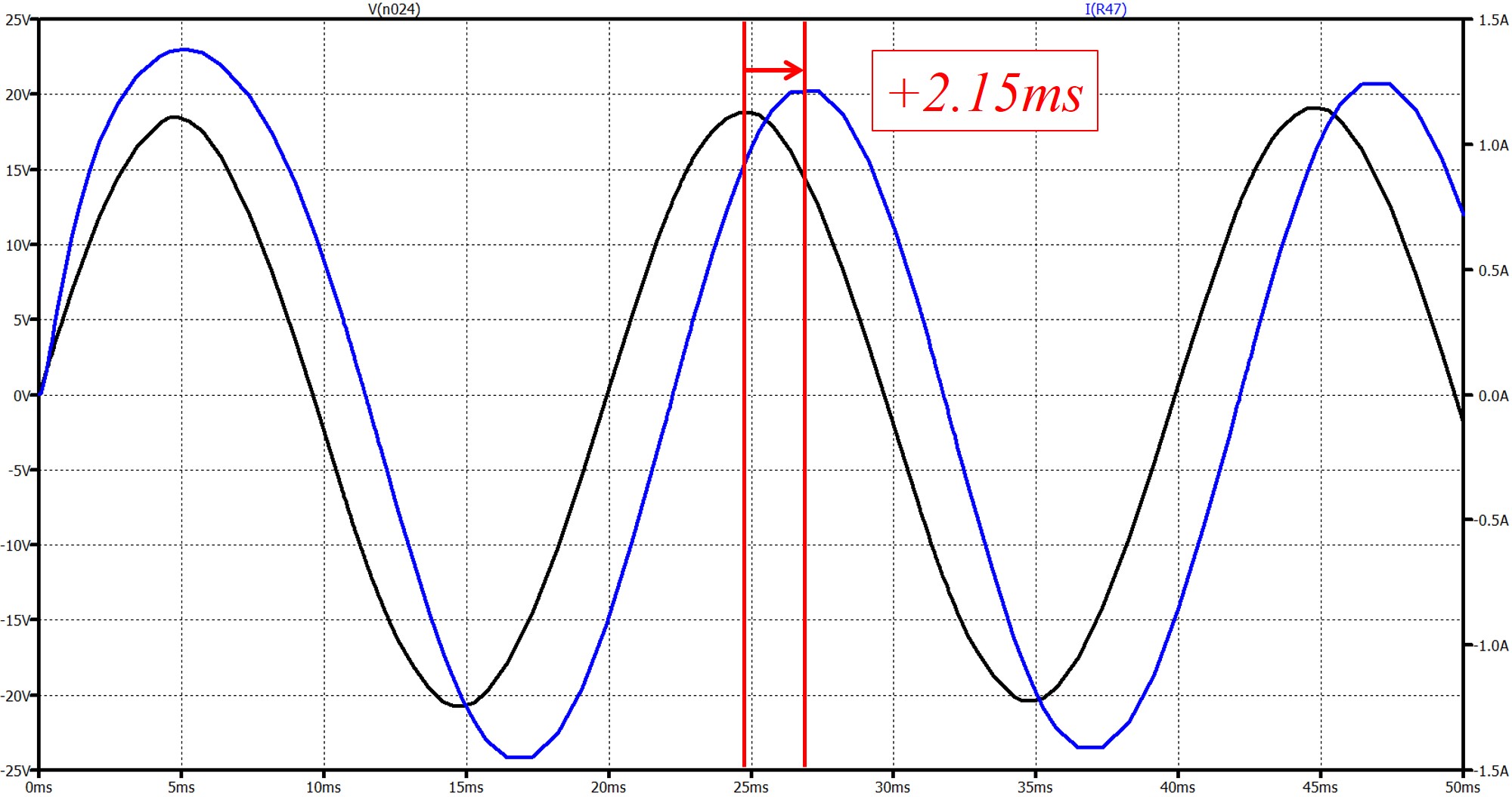
Here's an example. The plot shown below is a simulation of an audio amplifier output with a reactive load across its output terminals. The black trace is a 50Hz sine wave with an 18V amplitude applied to the load. The current waveform provided by the amplifier is shown in blue. After a few milliseconds of being turned on, the current waveform stabilizes to lead the voltage by 2.15ms. Given that it takes 20ms for a 50Hz sine wave to sweep through a single cycle (=360°), a 2.15ms leading current waveform corresponds to approximately a +39° (=+0.69 radians) phase angle between the two when referenced to the voltage.

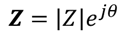
The relationship stated by the "Sparky" cartoon character is the polar (or exponential) expression of impedance, Z, and consists of the product of a scalar, Z, and a exponential function of the phase angle, q. It looks complicated but it's not. Impedance can also be expressed using the rectangular (or Cartesian) form:

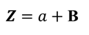where a is the resistance (a positive real number) and B is the reactance (an imaginary number) which can take on values of +jX, -jX or 0.

In the plot shown above, I'll show how the impedance of the load at 50Hz is determined. But first, the Nyquist plot is explained.

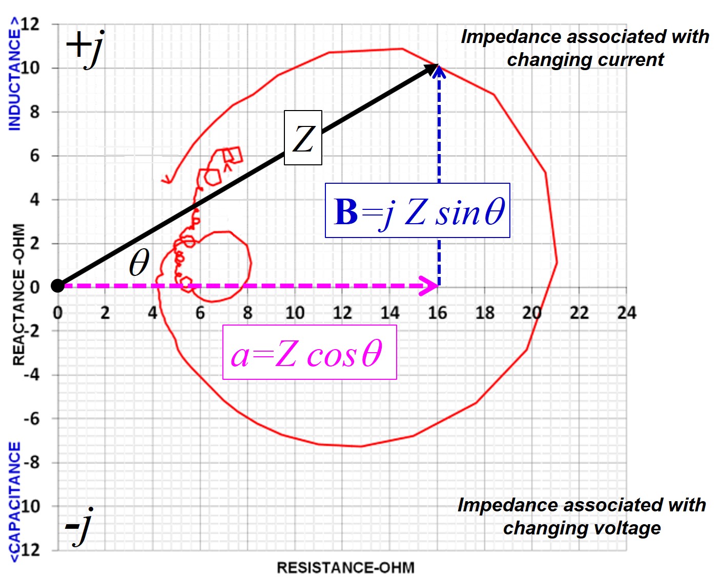
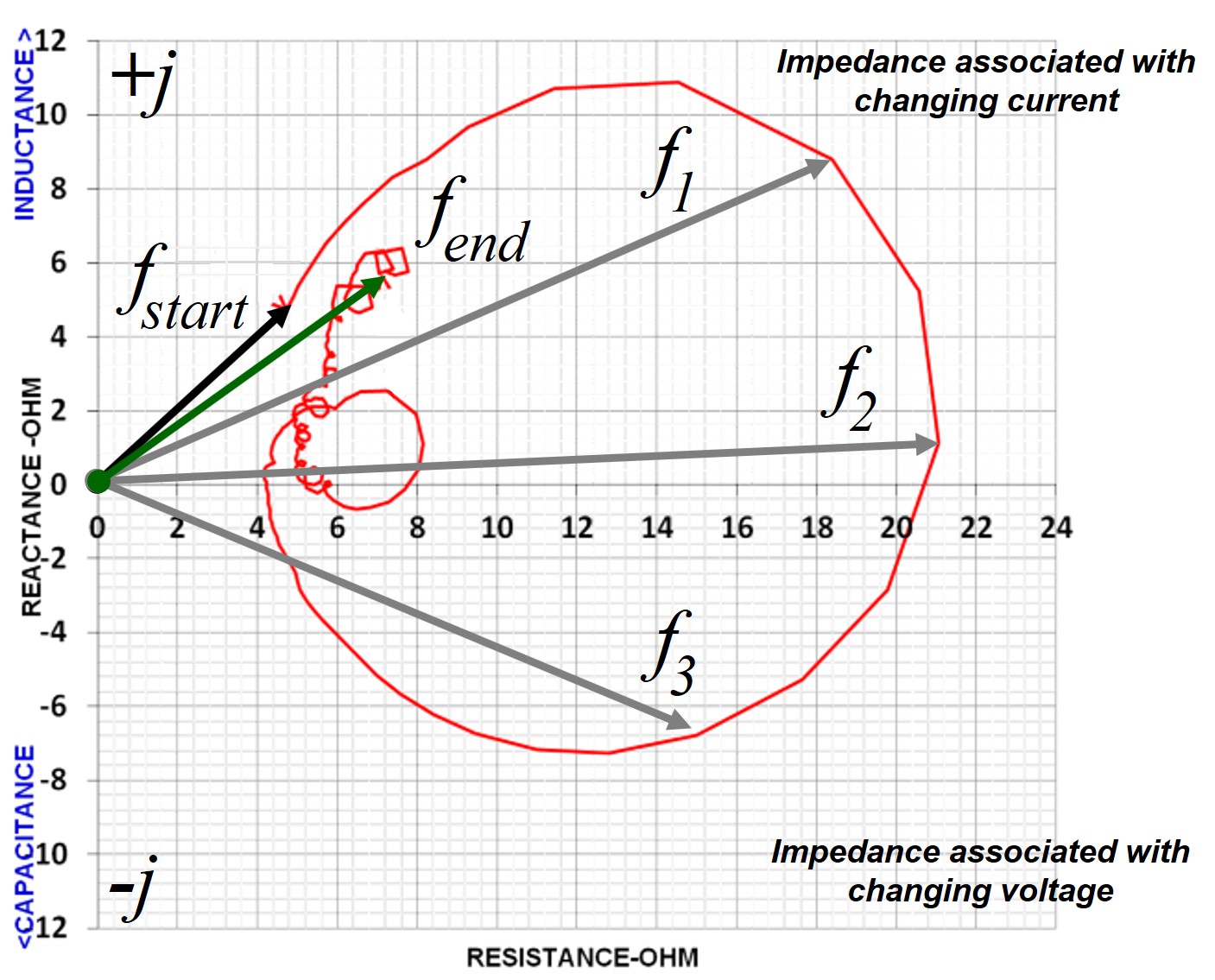
RECTANGULAR (CARTESIAN) AND POLAR (EXPONENTIAL) FORMS OF IMPEDANCE
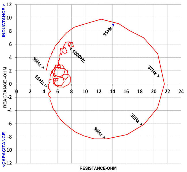
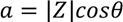
With regard to loudspeaker and audio filter engineering, the "nuts and bolts" of a Nyquist plot are shown below. The red trace is the impedance of a Klipschorn bass horn with no crossover filter between it and the amplifier. The trace represents the impedance plot between a start and end frequency. The black vector labeled Z has one end anchored at the origin and represents the hypotenuse of a right triangle with one leg projected along the X-axis (the real axis) and one leg parallel to j-axis (the imaginary axis). The location of the opposite end (arrowhead end) of the vector is determined by frequency and, as is shown in the adjacent plot, traces out the impedance continuously as the frequency is increased from the start to the end of the frequency range examined (fstart < f1 < f2 < f3 < fend). In the case of the Klipschorn plot shown the start frequency was 30Hz and the end frequency was 1000Hz. The length of the Z vector represents the impedance magnitude, the B leg represents the reactance and the a leg represents the resistance. The trigonometric forms of B and a are also shown.

Let's restate the exponential form of impedance:

.

Using the Euler relationship, the exponential function of phase angle can be expanded:

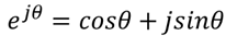
and, when substituted back into the exponential form and multiplied by IZI, becomes:

which demonstrates the exponential form of the impedance consists of the sum of a real and imaginary number. Thus, by observation and comparison to the rectangular form:

and

.

Thus, the rectangular form of the impedance is equal to:

and that's it for the equations.

THE j-OPERATOR
Consider the j-operator as a mathematical means to keep track of the type of reactance being sensed by the amplifier. A +j indicates an impedance associated with changes in current (inductive) whilst -j indicates impedance associated with changes in voltage (capacitive).

For example, a reactance of -j4.9 Ohms indicates that the current drawn by the load will lag the voltage provided by the amplifier and the load presents an impedance to the voltage source equal to 4.9 Ohms. To associate that to an "equivalent" capacitance however, the frequency must be known and a perfect 32.5uF capacitor would provide the 4.9 Ohms of reactance at 1000Hz (to prove it, go to any of a number of "reactance calculators" on the web that treat both capacitive and inductive loads). At 5000Hz, a 6.5uF capacitor would also provide 4.9 Ohms of reactance. And that's why it's called reactance, the magnitude changes as the frequency changes.

In reality, capacitors also present a resistance that's independent of frequency but let's ignore that.

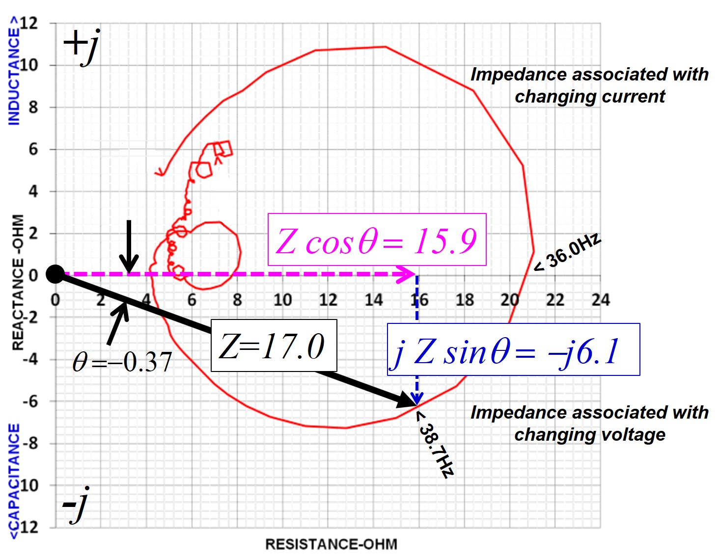
SOME EXAMPLES
Below are two examples showing how to read the impedance directly from the Nyquist plot. In the first, the magnitude vector is in the inductive (+j) quadrant and in the second plot the vector is in the capacitive (-j) quadrant. In the first, the magnitude of the impedance at 35.5Hz is 18.9 Ohms and consists of a 16 Ohm resistance and + j10.0 Ohm reactance. Expressed in rectangular form the impedance is Z = (16 + j10.0) Ohms at a frequency of 35.5Hz.

In the second plot, the magnitude vector is capacitive and has a magnitude of 17 Ohm, the resistance is 15.9 Ohm and the reactance is - j6.1 Ohm and, expressed in rectangular form, is Z = (15.9 - j6.1) Ohms at a frequency of 38.7Hz.

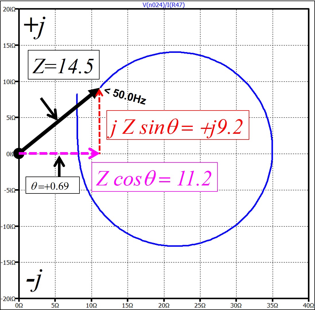
Now consider the impedance of the amplifier simulation shown earlier. Below is the simulated Nyquist plot of the impedance across the amplifier terminals between 50 and 1000Hz. At 50Hz the resistive part is 11.2 Ohm and the reactive part is +j9.2. The magnitude at 50Hz is 14.6 Ohms and the phase angle is +0.69 radians.

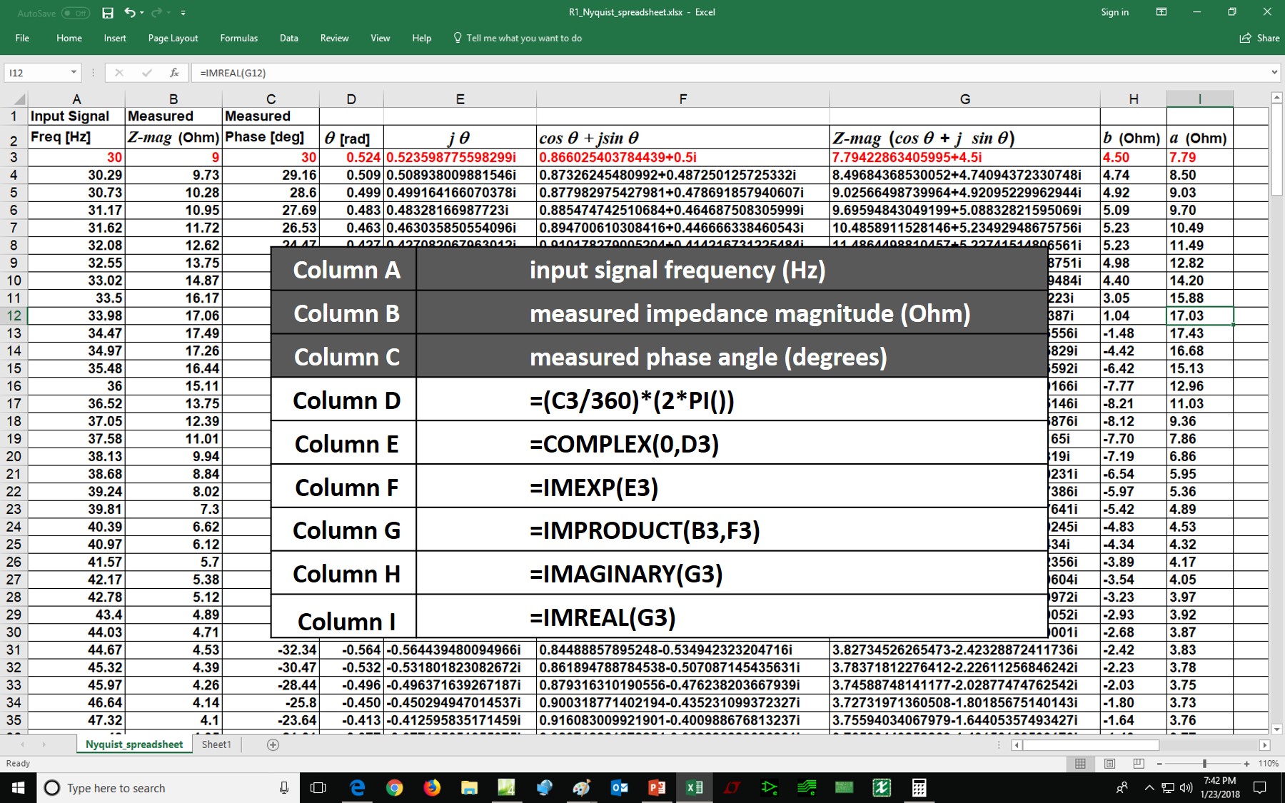
USING EXCEL
Mathematics aside, Excel is where we do the heavy lifting. The screen capture below is of an Excel spreadsheet that's set up to derive resistance and reactance values from frequency dependent impedance magnitude and phase angle data. Columns A, B and C are the experimentally obtained data and show the impedance magnitude and phase angle at each test signal frequency. The table superimposed over the spreadsheet shows the Excel complex number commands that correspond to the cells in columns D thru I. In this example one row is considered, row 3 (red highlight). The spreadsheet provides the values for a and b shown in the expression for the rectangular form of the impedance derived above. Note that early versions of Excel require the Analysis Toolpak to be enabled prior to working with complex numbers.

With a and b derived, a Nyquist plot can be generated by selecting Column H as the Y-axis data and Column I as the X-axis data keeping in mind that a +/- b really means +/- jb.

This webpage, "Sparky" cartoon figure, text and graphical content are property of North Reading Engineering, North Reading, MA 01864 USA. No part of the above work may be copied and published, in part or in total without written permission.